
Information Theoretic Approaches to Model Selection
Model Selection in a Nutshell
- The Frequentist P-Value testing framework emphasizes the evaluation of a single hypothesis - the null. We evaluate whether we reject the null.
- This is perfect for an experiment where we are evaluating clean causal links, or testing for a a predicted relationship in data.
- Often, though, we have multiple non-nested hypotheses, and wish to evaluate each. To do so we need a framework to compare the relative amount of information contained in each model and select the best model or models. We can then evaluate the individual parameters.
How complex a model do you need to be useful?

Some models are simple but good enough

More Complex Models are Not Always Better or Right

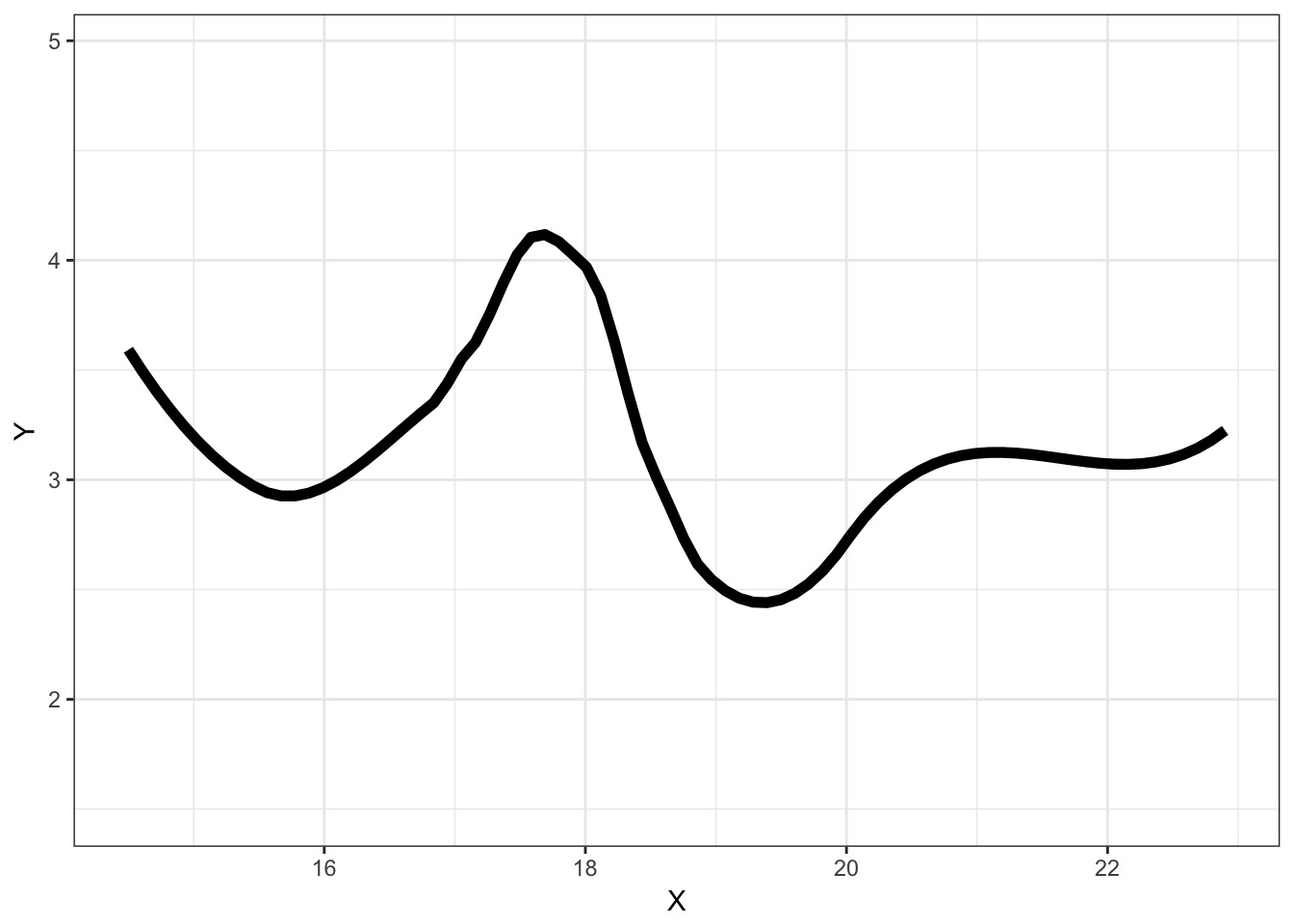
Consider this data…
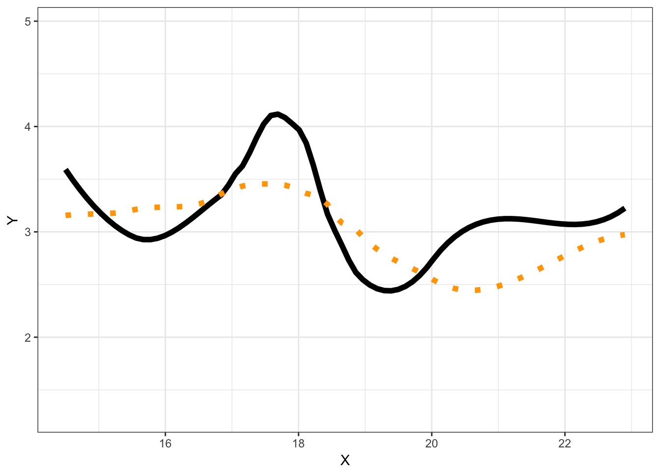
Underfitting
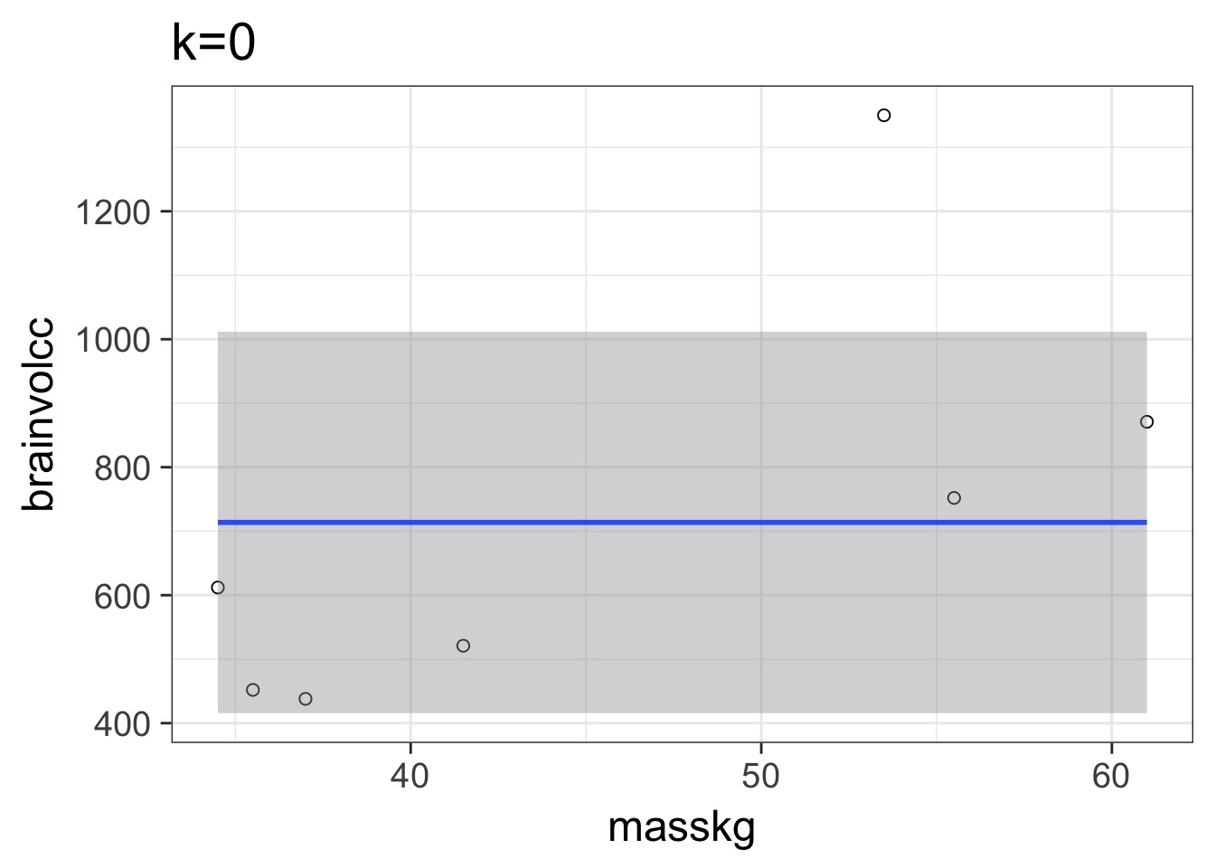
We have explained nothing!
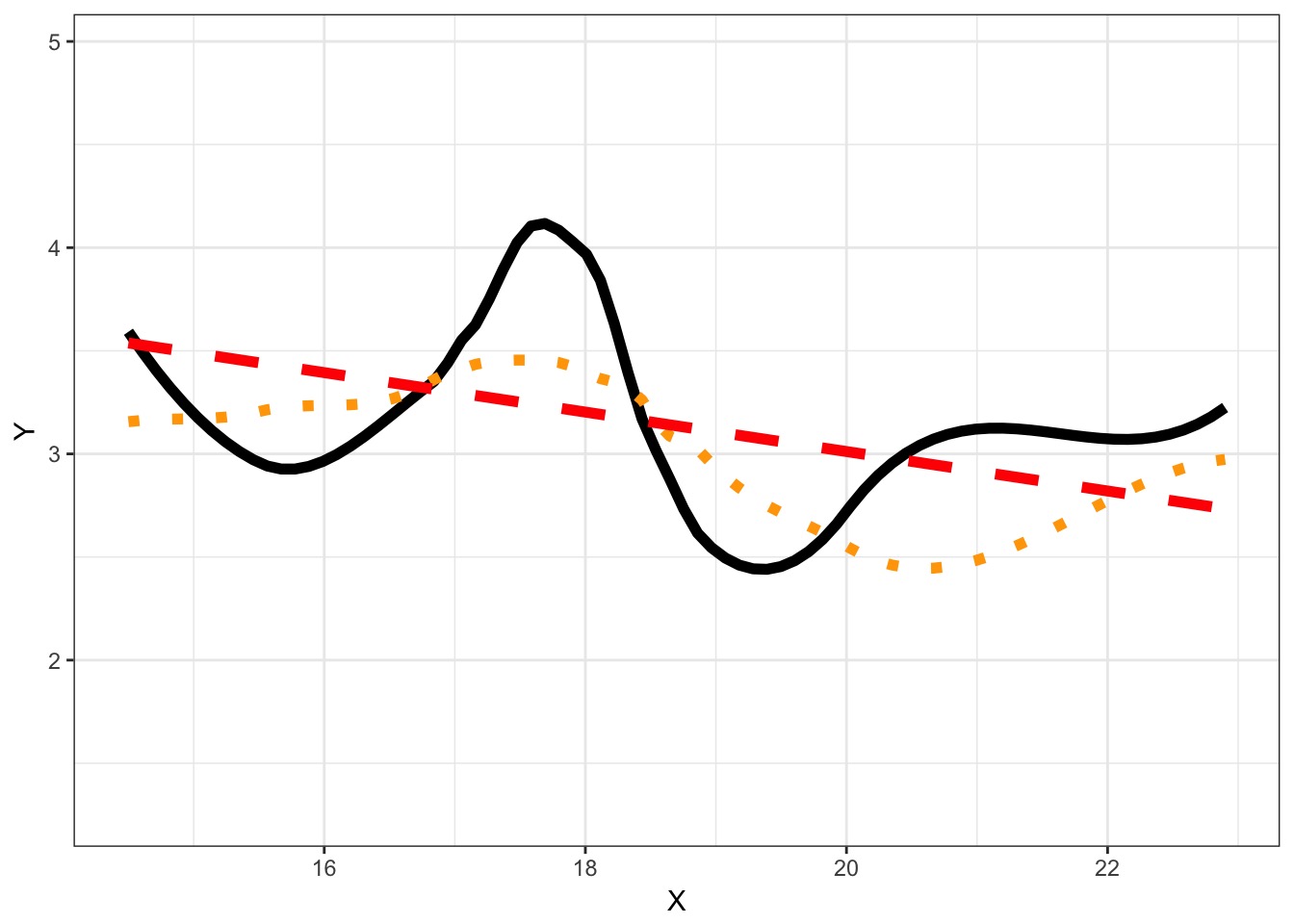
Overfitting
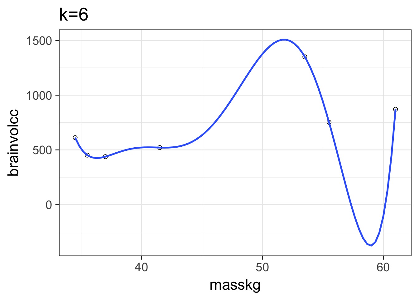
We have perfectly explained this sample
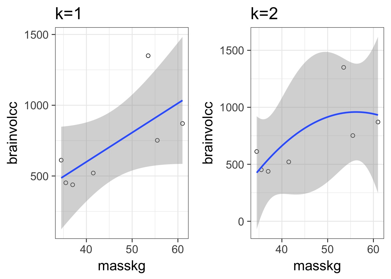
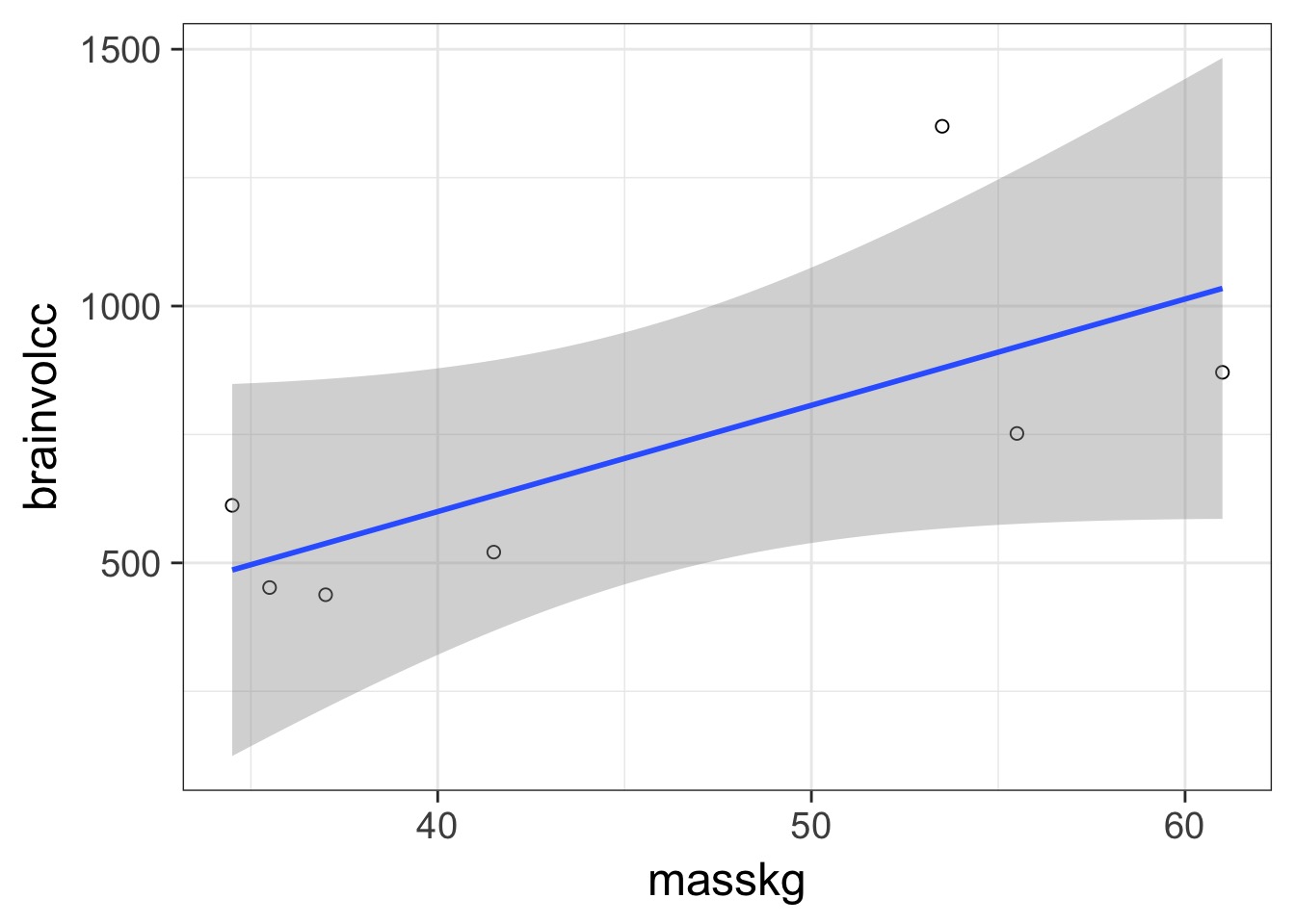
What is the right fit?
How do we Navigate?
- Regularization
- Penalize parameters with weak support
- Penalize parameters with weak support
- Optimization for Prediction
- Information Theory
- Draws from comparison of information loss
- Information Theory
In and Out of Sample Deviance
In and Out of Sample Deviance
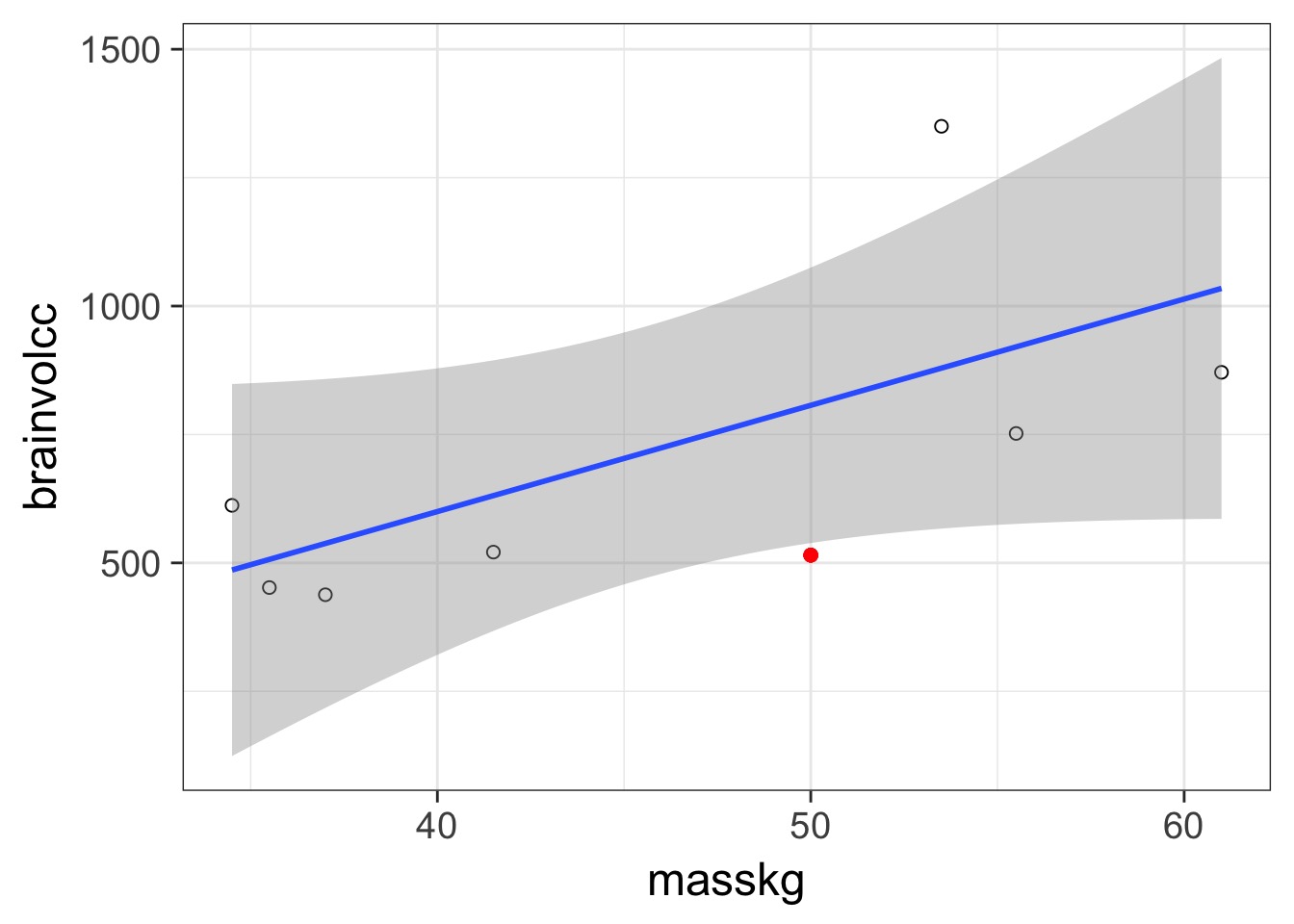
Prediction: 806.8141456, Observe: 515
Deviance: 8.526583810^{4}
In and Out of Sample Deviance
Our Goal for Judging Models
- Can we minimize the out of sample deviance
- So, fit a model, and evaluate how different the deviance is for a training versus test data set is
- What can we use to minimize the difference?
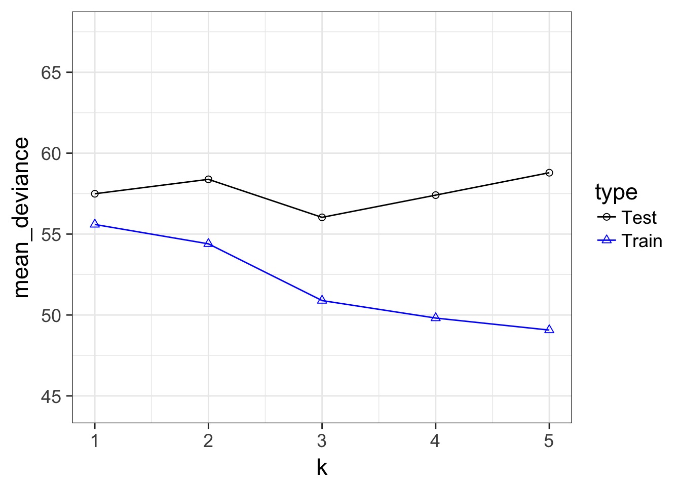
Train-Test Deviance
A Criteria Estimating Test Sample Deviance
- What if we could estimate out of sample deviance?
- The difference between training and testing deviance shows overfitting
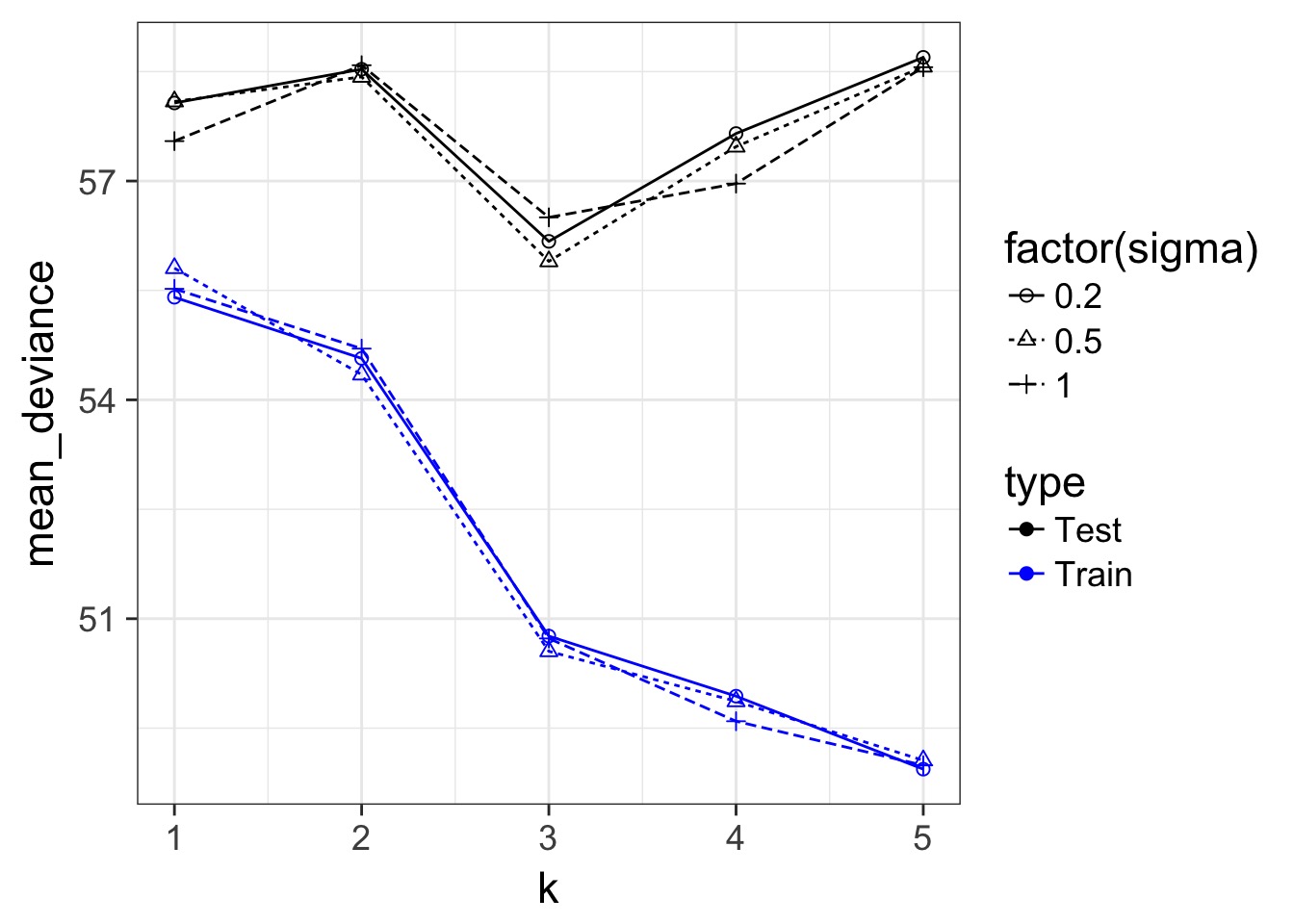
A Criteria Estimating Test Sample Deviance
 Slope here of 1.82
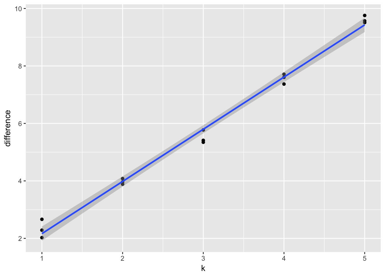
AIC

- So, \(E[D_{test}] = D_{train} + 2K\)
- This is Akaike’s Information Criteria (AIC)
\[AIC = Deviance + 2K\]
Suppose this is the Truth
We Can Fit a Model To Descibe Our Data, but it Has Less Information
We Can Fit a Model To Descibe Our Data, but it Has Less Information
Information Loss and Kullback-Leibler Divergence
Information Loss(truth,model) = L(truth)(LL(truth)-LL(model))
Two neat properties:
Comparing Information Loss between model1 and model2, truth drops out as a constant!
We can therefore define a metric to compare Relative Information Loss
Defining an Information Criterion
Akaike’s Information Criterion - lower AIC means less information is lost by a model \[AIC = -2log(L(\theta | x)) + 2K\]
Balancing General and Specific Truths
Which model better describes a general principle of how the world works? 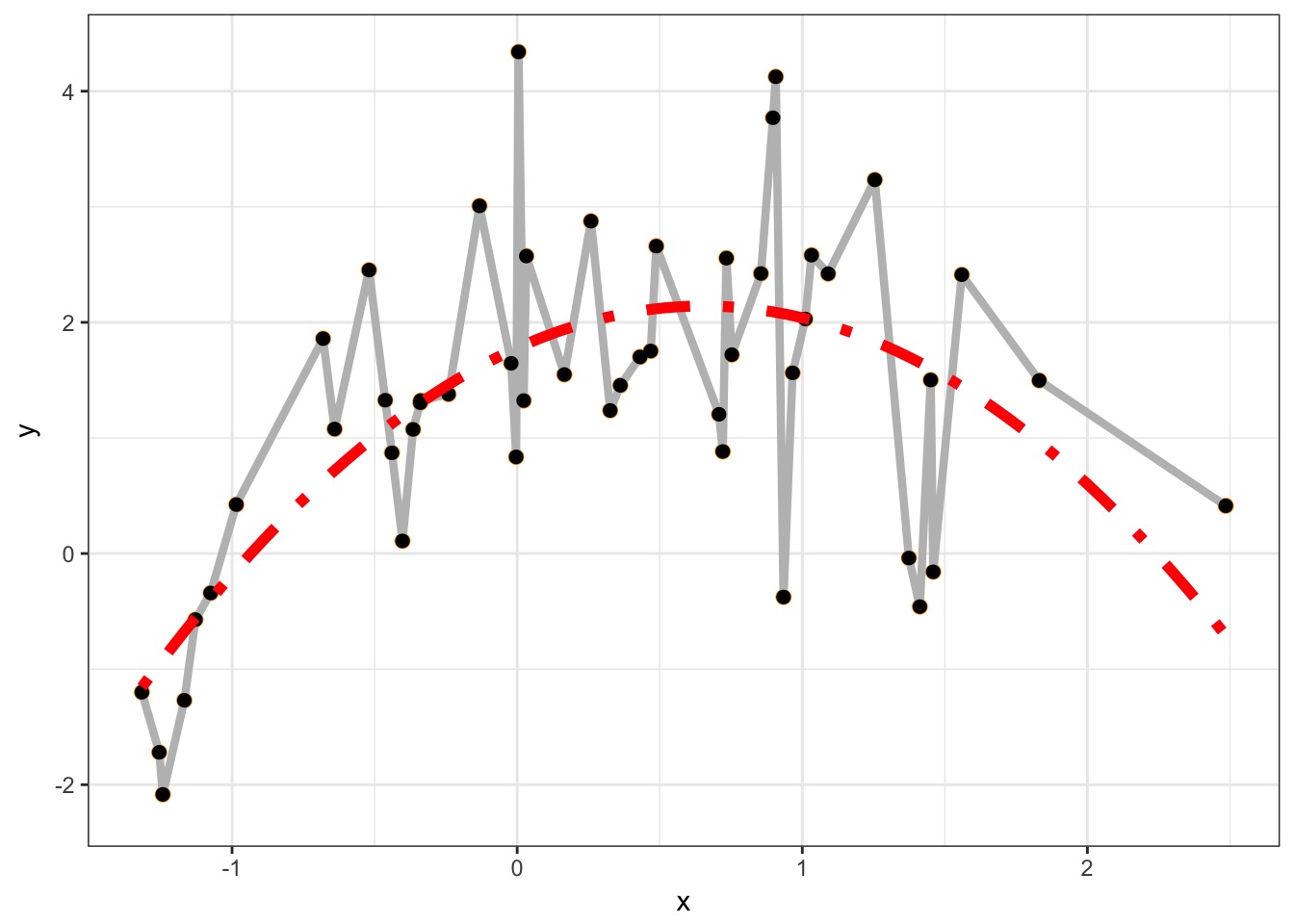
How many parameters does it take to draw an elephant?
AIC
- AIC optimized for forecasting (out of sample deviance)
- Assumes large N relative to K
- AICc for a correction
- AICc for a correction
But Sample Size Can Influence Fit…
\[AIC = -2log(L(\theta | x)) + 2K\]
\[AICc = AIC + \frac{2K(K+1)}{n-K-1}K\]
AIC v. BIC
Many other IC metrics for particular cases that deal with model complexity in different ways. For example \[AIC = -2log(L(\theta | x)) + 2K\]
Lowest AIC = Best Model for Predicting New Data
Tends to select models with many parameters
\[BIC = -2log(L(\theta | x)) + K ln(n)\]
Lowest BIC = Closest to Truth
- Derived from posterior probabilities
How can we Use AIC Values?
\[\Delta AIC = AIC_{i} - min(AIC)\]Rules of Thumb from Burnham and Anderson(2002):
- \(\Delta\) AIC \(<\) 2 implies that two models are similar in their fit to the data
- \(\Delta\) AIC between 3 and 7 indicate moderate, but less, support for retaining a model
- \(\Delta\) AIC \(>\) 10 indicates that the model is very unlikely
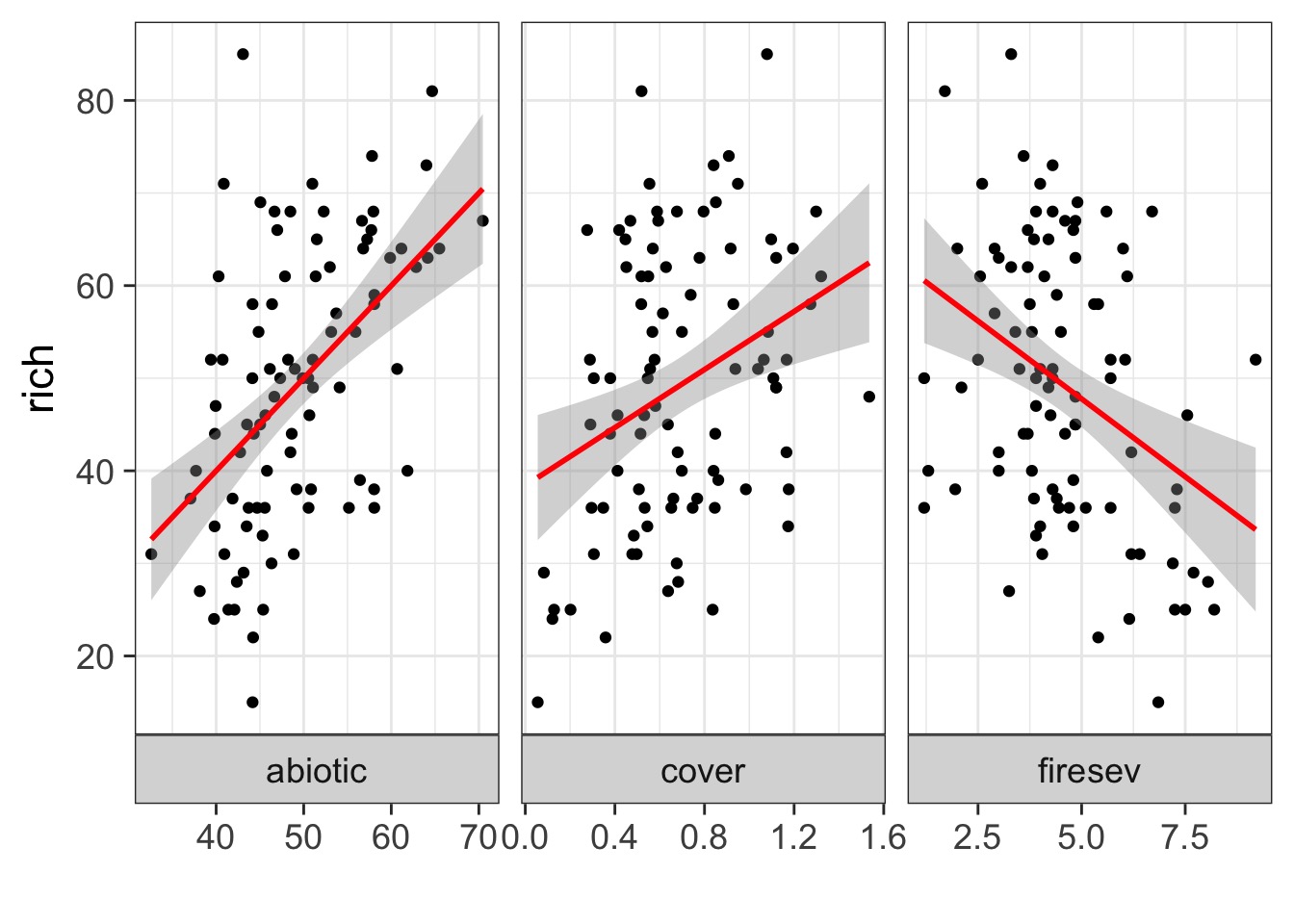
What causes species richness?
- Distance from fire patch
- Elevation
- Abiotic index
- Patch age
- Patch heterogeneity
- Severity of last fire
- Plant cover
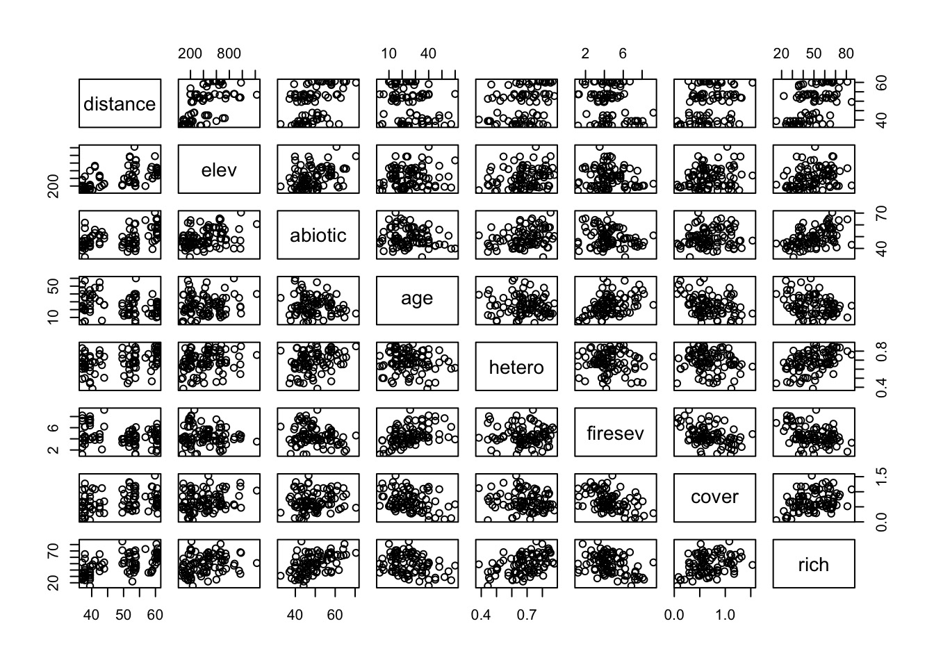
Many Things may Influence Species Richness
Implementing AIC: Create Models
Implementing AIC: Compare Models
[1] 722.2085[1] 736.0338[1] 738.796What if You Have a LOT of Potential Drivers?
7 models alone with 1 term each
127 possible without interactions.

A Quantitative Measure of Relative Support
\[w_{i} = \frac{e^{\Delta_{i}/2 }}{\displaystyle \sum^R_{r=1} e^{\Delta_{i}/2 }}\]
Where \(w_{i}\) is the relative support for model i compared to other models in the set being considered.
Model weights summed together = 1
Begin with a Full Model
We use this model as a jumping off point, and construct a series of nested models with subsets of the variables.
Evaluate using AICc Weights!
Models with groups of variables
One Factor Models
Null Model
Now Compare Models Weights
| Modnames | K | AICc | Delta_AICc | ModelLik | AICcWt | LL | |
|---|---|---|---|---|---|---|---|
| 1 | full | 9 | 688.162 | 0.000 | 1.000 | 0.888 | -333.956 |
| 3 | soil_fire | 7 | 692.554 | 4.392 | 0.111 | 0.099 | -338.594 |
| 4 | soil_plant | 7 | 696.569 | 8.406 | 0.015 | 0.013 | -340.601 |
| 7 | fire | 4 | 707.493 | 19.331 | 0.000 | 0.000 | -349.511 |
| 2 | plant_fire | 6 | 709.688 | 21.526 | 0.000 | 0.000 | -348.338 |
| 5 | soil | 5 | 711.726 | 23.564 | 0.000 | 0.000 | -350.506 |
| 6 | plant | 4 | 737.163 | 49.001 | 0.000 | 0.000 | -364.346 |
| 8 | null | 2 | 747.254 | 59.092 | 0.000 | 0.000 | -371.558 |
So, I have some sense of good models? What now?

Variable Weights
How to I evaluate the importance of a variable?
Variable Weight = sum of all weights of all models including a variable. Relative support for inclusion of parameter in models.
Importance values of 'firesev':

w+ (models including parameter): 0.99
w- (models excluding parameter): 0.01

Model Averaged Parameters
\[\hat{\bar{\beta}} = \frac{\sum w_{i}\hat\beta_{i}}{\sum{w_i}}\]
\[var(\hat{\bar{\beta}}) = \left [ w_{i} \sqrt{var(\hat\beta_{i}) + (\hat\beta_{i}-\hat{\bar{\beta_{i}}})^2} \right ]^2\]
Buckland et al. 1997
Model Averaged Parameters
Multimodel inference on "firesev" based on AICc

AICc table used to obtain model-averaged estimate with shrinkage:

           K   AICc Delta_AICc AICcWt Estimate   SE
full       9 688.16       0.00   0.89    -1.02 0.80
plant_fire 6 709.69      21.53   0.00    -1.39 0.92
soil_fire  7 692.55       4.39   0.10    -1.89 0.73
soil_plant 7 696.57       8.41   0.01     0.00 0.00
soil       5 711.73      23.56   0.00     0.00 0.00
plant      4 737.16      49.00   0.00     0.00 0.00
fire       4 707.49      19.33   0.00    -2.03 0.80
null       2 747.25      59.09   0.00     0.00 0.00

Model-averaged estimate with shrinkage: -1.09
Unconditional SE: 0.84
95% Unconditional confidence interval: -2.74, 0.56

Model Averaged Predictions
newData <- data.frame(distance = 50,
                      elev = 400,
                      abiotic = 48,
                      age = 2,
                      hetero = 0.5,
                      firesev = 10,
                      cover=0.4)
Model-averaged predictions on the response scale
based on entire model set and 95% confidence interval:

  mod.avg.pred uncond.se lower.CL upper.CL
1       31.666     6.136    19.64   43.692
Death to model selection
- While sometimes the model you should use is clear, more often it is not
- Further, you made those models for a reason: you suspect those terms are important
- Better to look at coefficients across models
- For actual predictions, ensemble predictions provide real uncertainty
Ensemble Prediction
- Ensemble prediction gives us better uncertainty estimates
- Takes relative weights of predictions into account
- Takes weights of coefficients into account
- Basicaly, get simulated predicted values, multiply them by model weight
Cautionary Notes
AIC analyses aid in model selection. One must still evaluate parameters and parameter error.
Your inferences are constrained solely to the range of models you consider. You may have missed the ’best’ model.
All inferences MUST be based on a priori models. Post-hoc model dredging could result in an erroneous ’best’ model suited to your unique data set.