Generalized Linear Models

Surival in the Zoo

Survival Data is often nonlinear and not normal

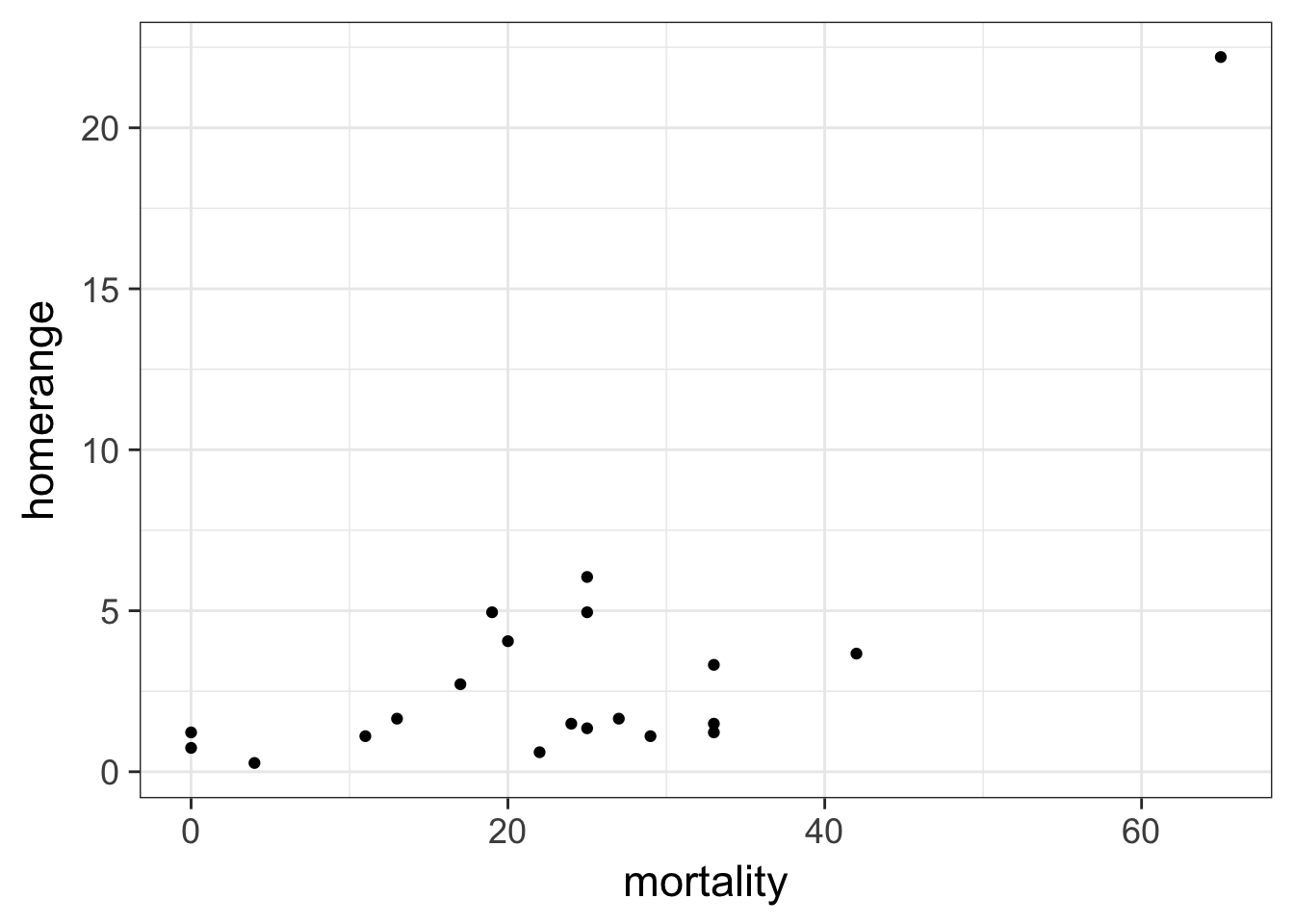
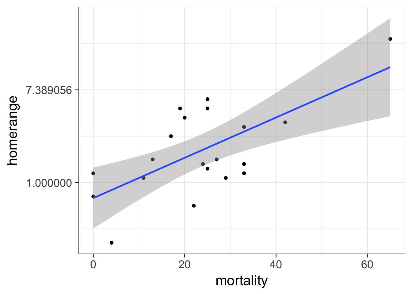
We can transform…

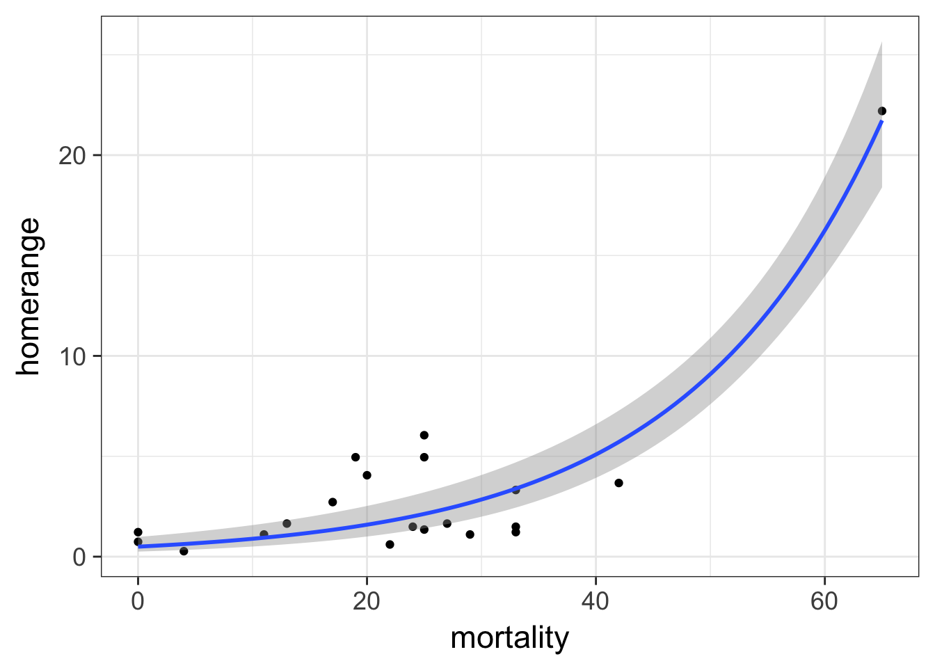
But non-normal error generating process are also common

The General Linear Model

\[\Large \boldsymbol{Y_i} = \boldsymbol{\beta X_i} + \boldsymbol{\epsilon} \]





\[\Large \epsilon \sim \mathcal{N}(0,\sigma^{2})\]

The General(ized) Linear Model

\[\Large \boldsymbol{\hat{Y}_{i}} = \boldsymbol{\beta X_i} \]





\[\Large Y_i \sim \mathcal{N}(\hat{Y_i},\sigma^{2})\]

The General(ized) Linear Model

\[\Large \boldsymbol{\eta_{i}} = \boldsymbol{\beta X_i} \]

\[\Large \hat{Y_i} = \eta_{i}\] Identity Link Function

\[\Large Y_i \sim \mathcal{N}(\hat{Y_i},\sigma^{2})\]

A Generalized Linear Model

\[\Large \boldsymbol{\eta_{i}} = \boldsymbol{\beta X_i} \]

\[\Large Log(\hat{Y_i}) = \eta_{i}\] Log Link Function

\[\Large Y_i \sim \mathcal{N}(\hat{Y_i},\sigma^{2})\]

Generalized Linear Models Errors

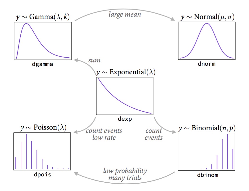
Connections Between Errors

Generalized Linear Models Errors

Log-Normal Distributions

\[ Y_i \sim LN(\mu, \sigma^2)\]

• Used for data whose error is additive, but from multiplicative process
  
  
• \(Y_i = e^X + e^{\epsilon_i}, \epsilon_i \sim N(0, \sigma^2)\)
  - Error is additive
  - E.g. variance is from external sources, happens to be LN
  
  
• This is very different form a log transform
  
  
• \(Y_i = e^{x}e^{\epsilon_i}\)
  - Error is multiplicative
  - E.g., variance is something that accumulates over time

The GLM

zoo_mod <- glm(homerange ~ mortality, data=zoo,
               family=gaussian(link="log"))

Our two big questions

1. Does our model explain more variation in the data than a null model?
   
   
2. Are the parameters different from 0?

Evaluating the DGP: \(\chi^2\) Likelihood Ratios

• We fit GLMs using different techniques
  
  
• A model has a Likelihood of the model given the data
  
  
• The ratio of the likelihood of the model versus the likelihood of a null model is \(\chi^2\) distributed
  
  
• It’s like an F test, but with Likelihoods instead of Mean Squares
  
  

\(\chi^2\) Likelihood Ratios

library(car)
Anova(zoo_mod)

## Analysis of Deviance Table (Type II tests)
## 
## Response: homerange
##           LR Chisq Df Pr(>Chisq)    
## mortality   105.68  1  < 2.2e-16 ***
## ---
## Signif. codes:  0 '***' 0.001 '**' 0.01 '*' 0.05 '.' 0.1 ' ' 1

Plotting with stat_smooth and glms

home +
  stat_smooth(method="glm", 
              method.args=list(family=gaussian(link="log")))

Plotting with stat_smooth and glms

Generalized Linear Models Errors

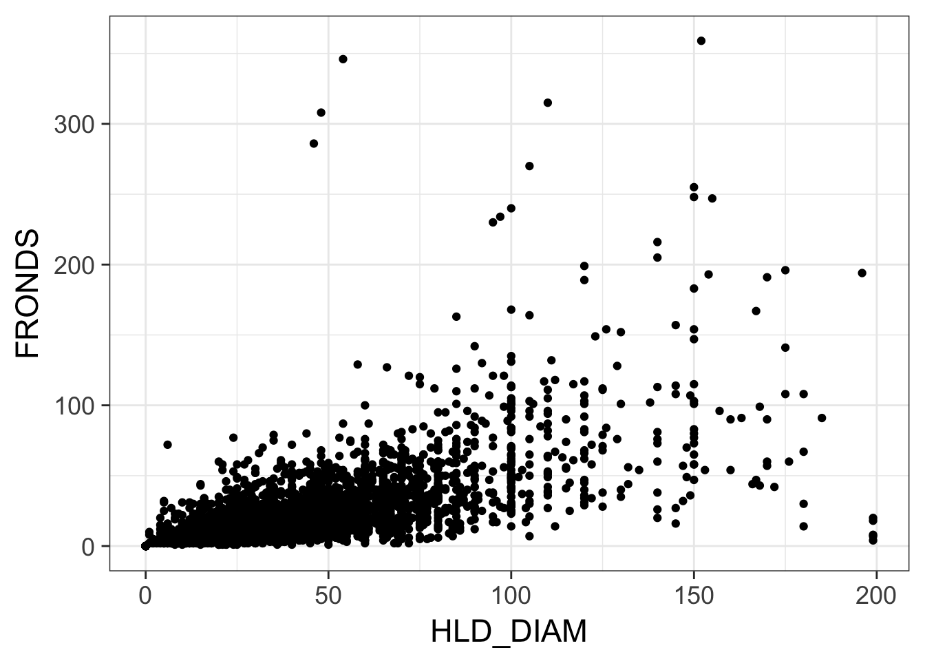
Does Size of Holdfast Matter?

• Kelps are held to rock by holdfasts
• Older kelps have bigger holdfasts
• Does size of holdfast influence number of stipes from kelp?

Does Size of Holdfast Matter?

Poisson Distributions

\[Y_i \sim P(\lambda)\]

• Discrete Distribution
  
  
• Used for count data
  
  
• \(\lambda\) = mean
  
  
• Variance increases linearly with mean
  
  

The GLM

kelp_mod <- glm(FRONDS ~ HLD_DIAM, data=kelp,
               family=poisson(link="log"))

Fit

kelp_plot +
  stat_smooth(method="glm", method.args=(family=poisson))

Generalized Linear Models Errors

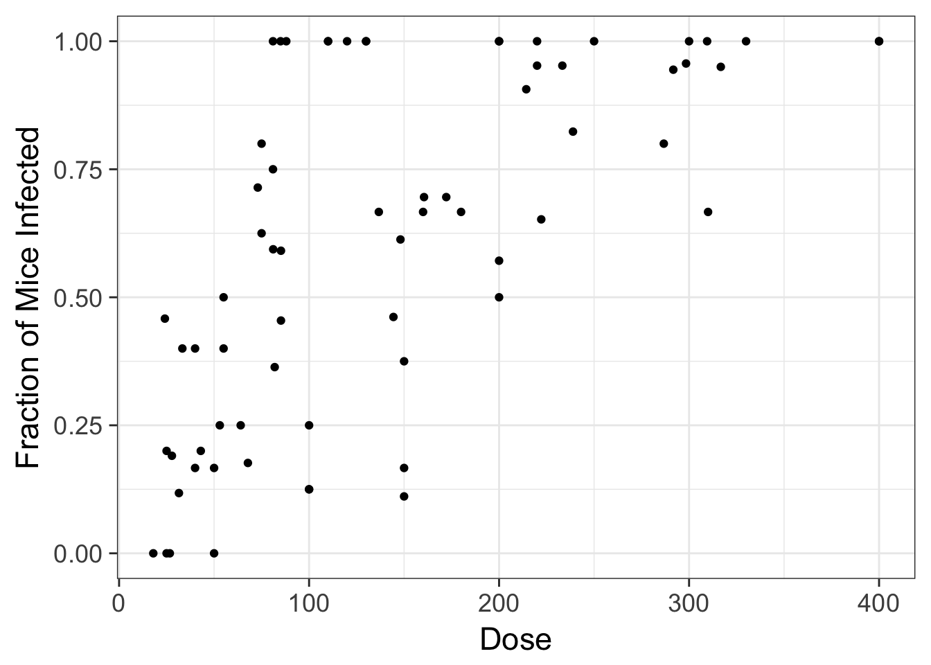
Cryptosporidum Infection Rates

Binomial Distribution

\[ Y_i \sim B(prob, size) \]

• Discrete Distribution
  
  
• prob = probability of something happening
  
  
• size = # of discrete trials
  
  
• Used for frequency or probability data
  
  
• We estimate coefficients that influence prob
  
  

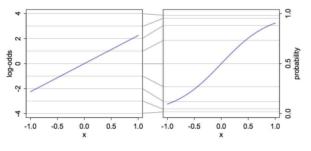
Generalized Linear Model with a Logit Link

\[\Large \boldsymbol{\eta_{i}} = \boldsymbol{\beta X_i} \]

\[\Large Logit(\hat{Y_i}) = \eta_{i}\] Logit Link Function

\[\Large Y_i \sim \mathcal{B}(\hat{Y_i}, size)\]

Logit Link

McElreath’s Statistical Rethinking

Logitistic Regression

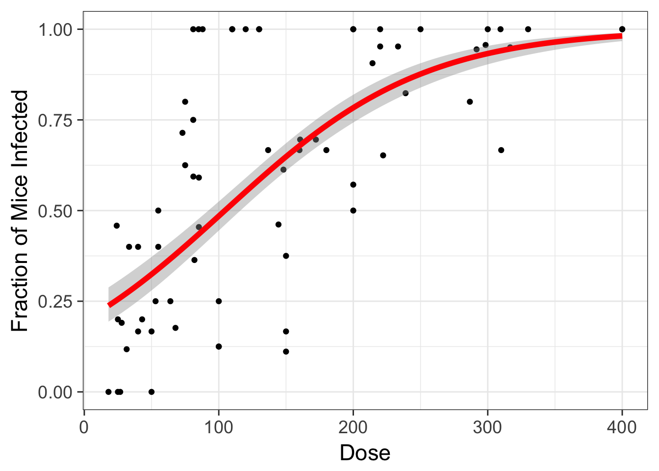
Generalized Linear Model with Logit Link

crypto_glm <- glm(Y/N ~ Dose,
                  weight=N,
                  family=binomial(link="logit"),
                  data=crypto)

OR, with Success and Failures

crypto_glm <- glm(cbind(Y, Y-N) ~ Dose,
                  family=binomial(link="logit"),
                  data=crypto)

Outputs

And logit coefficients

Generalized Linear Models Errors

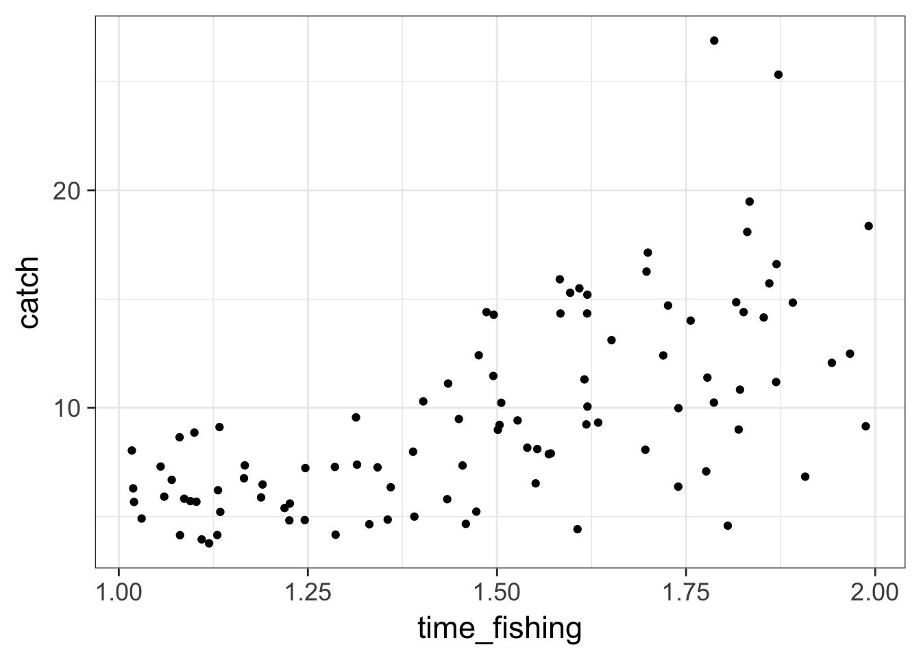
How long should you fish?

Example from http://seananderson.ca/2014/04/08/gamma-glms/

Mo’ Fish = Mo’ Variance

The Gamma Distribution

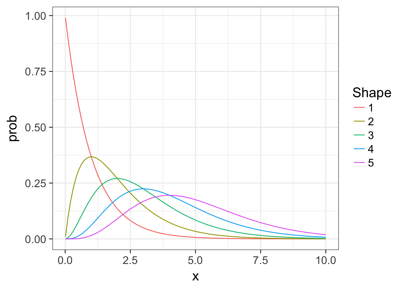
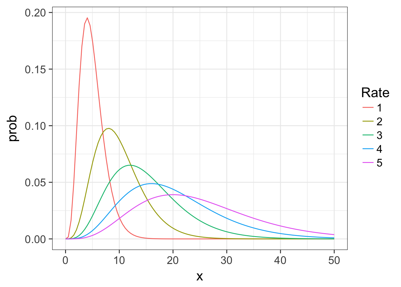
\[Y_i \sim Gamma(shape, scale)\]

• Continuous Distribution, bounded at 0
  
  
• Used for time data
  
  
• \(shape\) = number of events waiting for
  
  
• \(scale\) = time for one event
  
  
• Variance increases with square mean
  
  

The Gamma Distribution: Rate = 1

The Gamma Distribution: Shape = 5

The Gamma Distribution in Terms of Fit

\[Y_i \sim Gamma(shape, scale)\]

For a fit value \(\hat{Y_i}\):

• \(shape = \frac{\hat{Y_i}}{scale}\)
  
  
• \(scale = \frac{\hat{Y_i}}{shape}\)
  
  
• Variance = \(shape \cdot scale^2\)

The Gamma Fit with a Log Link

Gamma Fit on a Plot

fish_plot +
  stat_smooth(method = "glm", 
              method.args=list(family=Gamma(link="log")),  
              col="red", lwd=2)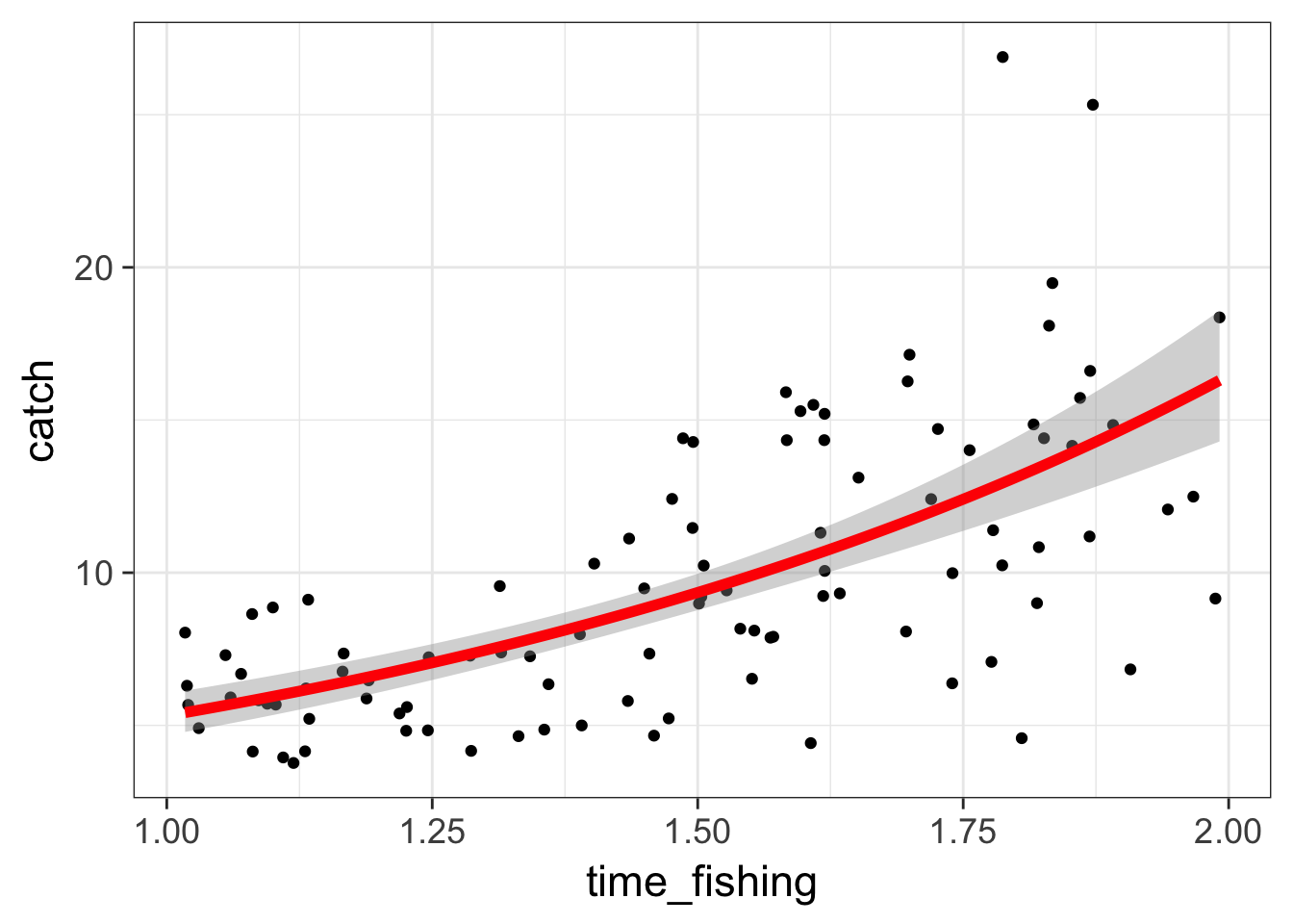 

How to Choose Among GLMs

1. Is your data continuous or count
   
   
2. How does the variance scale with the mean?
   
   
3. What is the shape of your relationship from the DGP?