Making Data Tell its Story

Where are we going?

Groups of Topics

1. Our Data

2. Cleaning and Filtering our Data

3. Summarizing counts functionally!

4. How do we summarize our data?

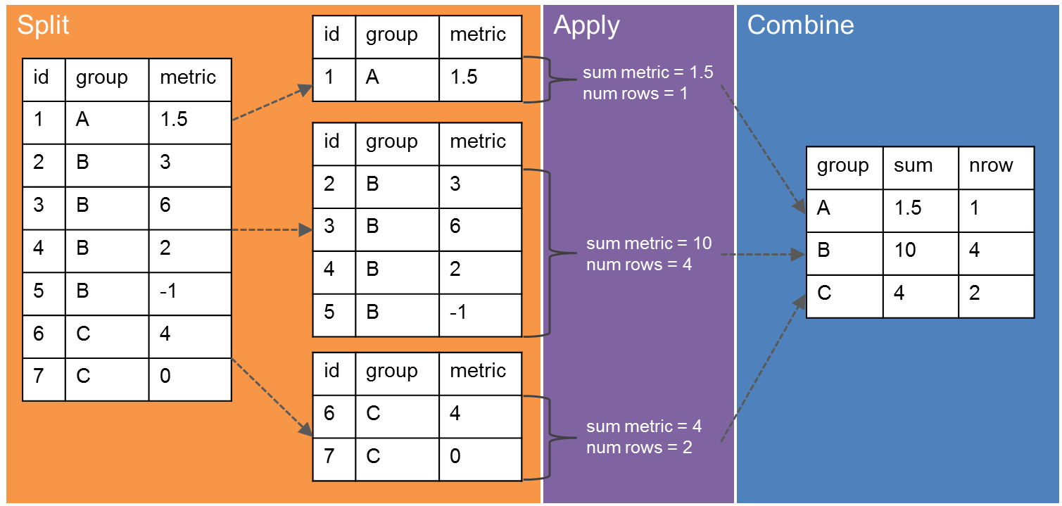
5. The split-apply-combine philosophy

How much does one salmon weigh?

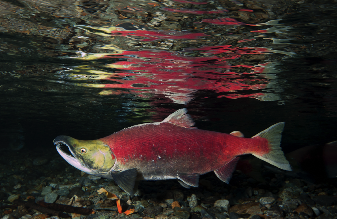
Weight: 3.09kg

How much do these salmon weigh?

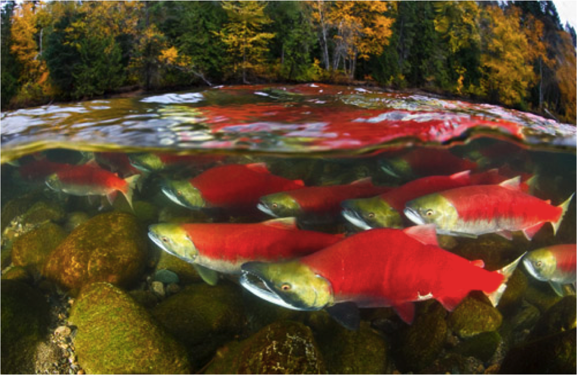
3.09, 2.91, 3.06, 2.69, 2.88, 2.98, 1.61, 2.16, 1.56, 1.76

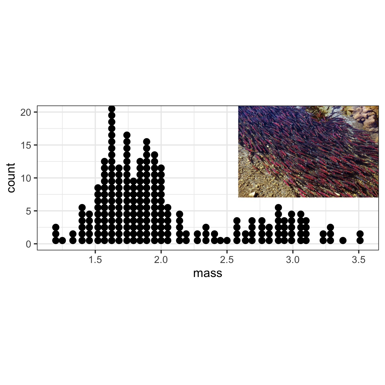
What can we say about the weights of all of these salmon?

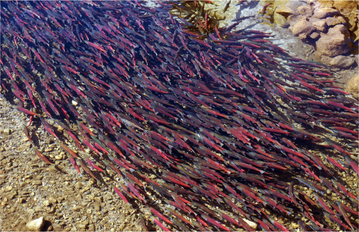
Pair up with someone and come up all of the information you can think of that would summarize this population.

Our Data

Groups of Topics

1. Our Data

2. Cleaning and Filtering our Data

3. Summarizing counts functionally!

4. How do we summarize our data?

5. The split-apply-combine philosophy

What Data Do We Want?

What Data Do We Want? Adults!

Our Hero…

Filtering

library(dplyr)

filter(salmon, mass > 2)

# A tibble: 74 × 3
    mass river mass_class 
   <dbl> <chr> <fct>      
 1  3.09 a     (2.75,3.14]
 2  2.91 b     (2.75,3.14]
 3  3.06 c     (2.75,3.14]
 4  2.69 d     (2.35,2.75]
 5  2.88 e     (2.75,3.14]
 6  2.98 f     (2.75,3.14]
 7  2.16 b     (1.96,2.35]
 8  3.3  f     (3.14,3.53]
 9  3.25 e     (3.14,3.53]
10  2.18 f     (1.96,2.35]
# ℹ 64 more rows

Filtering

filter(salmon, river == "a")

# A tibble: 38 × 3
    mass river mass_class 
   <dbl> <chr> <fct>      
 1  3.09 a     (2.75,3.14]
 2  1.61 a     (1.57,1.96]
 3  1.91 a     (1.57,1.96]
 4  2.13 a     (1.96,2.35]
 5  1.53 a     [1.18,1.57]
 6  1.75 a     (1.57,1.96]
 7  1.76 a     (1.57,1.96]
 8  1.72 a     (1.57,1.96]
 9  2.29 a     (1.96,2.35]
10  1.74 a     (1.57,1.96]
# ℹ 28 more rows

Logical Operators

Many Filters

filter(salmon, river == "a" & mass > 3)

# A tibble: 4 × 3
   mass river mass_class 
  <dbl> <chr> <fct>      
1  3.09 a     (2.75,3.14]
2  3.04 a     (2.75,3.14]
3  3.11 a     (2.75,3.14]
4  3.05 a     (2.75,3.14]

Groups of Topics

1. Our Data

2. Cleaning and Filtering our Data

3. Summarizing counts functionally!

4. How do we summarize our data?

5. The split-apply-combine philosophy

Counting

# A tibble: 1 × 1
      n
  <int>
1   228

Nesting Functions: Ugly! Hard to Read!

count( filter(salmon, river == "a" & mass > 3) )

# A tibble: 1 × 1
      n
  <int>
1     4

Introducing The Pipe

filter(salmon, river == "a" & mass > 3) |>
  count()

# A tibble: 1 × 1
      n
  <int>
1     4

Sidebar - the pipe!

Sidebar - the pipe!

Pipes pass an object as the first argument to a function

5 |> sum(4)

[1] 9

salmon |> count()

# A tibble: 1 × 1
      n
  <int>
1   228

Pipes and Functional Programming

• We often thing in terms of do this, then then, then this
  
  
• Programming that way requires overwriting a lot of objects
  
  
• It gets…. messy

Functional Programming Workflow

#filter the salmon data by river

#filter the salmon data by mass

#get the count of the salmon

Functional Programming Can get Verbose

#filter the salmon data by river
salmon_filtered <- filter(salmon, river == "a") 

#filter the salmon data by mass
salmon_filtered <- filter(salmon_filtered, mass > 3) 

#get the count of the salmon
count(salmon_filtered)

Pipes Make Programs Read Like Language!

salmon_filtered <- salmon |>
  
  #filter the salmon data by river
  filter(river == "a") |>
  
  #filter the salmon data by mass
  filter(mass > 3) |>
  
  #get the count of the salmon
  count()

Groups of Topics

1. Our Data

2. Cleaning and Filtering our Data

3. Summarizing counts functionally!

4. How do we summarize our data?

5. The split-apply-combine philosophy

Summary Properties of a Sample

• Measures of Central tendency: Mean, Median, Mode

• Measures of Variation: Standard Deviation, Percentiles

• Measures of Precision of Estimating the Above: Standard Error

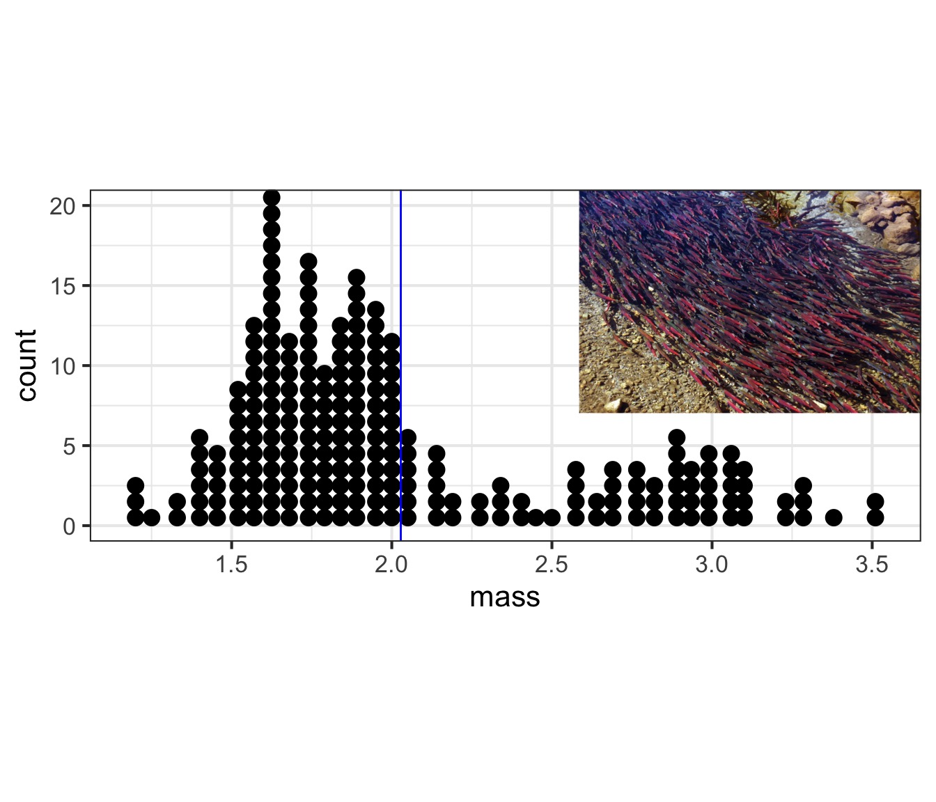
Median - Dead Center

 [1] 1.56 1.61 1.76 2.16 2.69 2.88 2.91 2.98 3.06 3.09

[1] 1.855

Central Tendancies

What about population-level variability?

What about population-level variability? 2/3 of the population is within 1SD

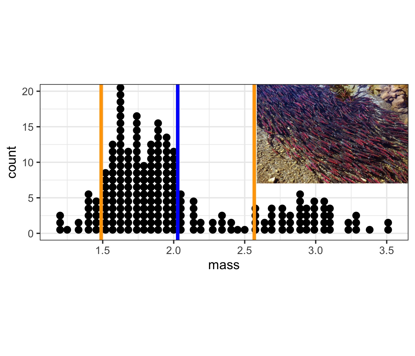
What is the range of 2/3 of the population?

Sample Properties: Variance

How variable was that population? \[\large s^2= \frac{\displaystyle \sum_{i=1}^{n}{(Y_i - \bar{Y})^2}} {n-1}\]

• Sums of Squares over n-1
  
• n-1 corrects for both sample size and sample bias
  
• Units in square of measurement…

Sample Properties: Standard Deviation

\[ \large s = \sqrt{s^2}\]

• Units the same as the measurement
• If distribution is normal, 67% of data within 1 SD
• 95% within 2 SD

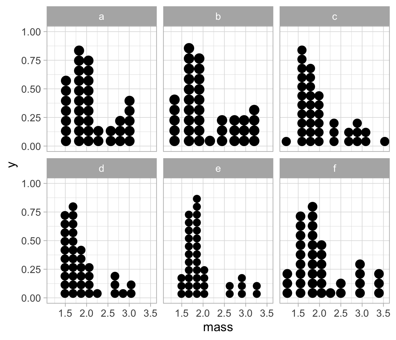
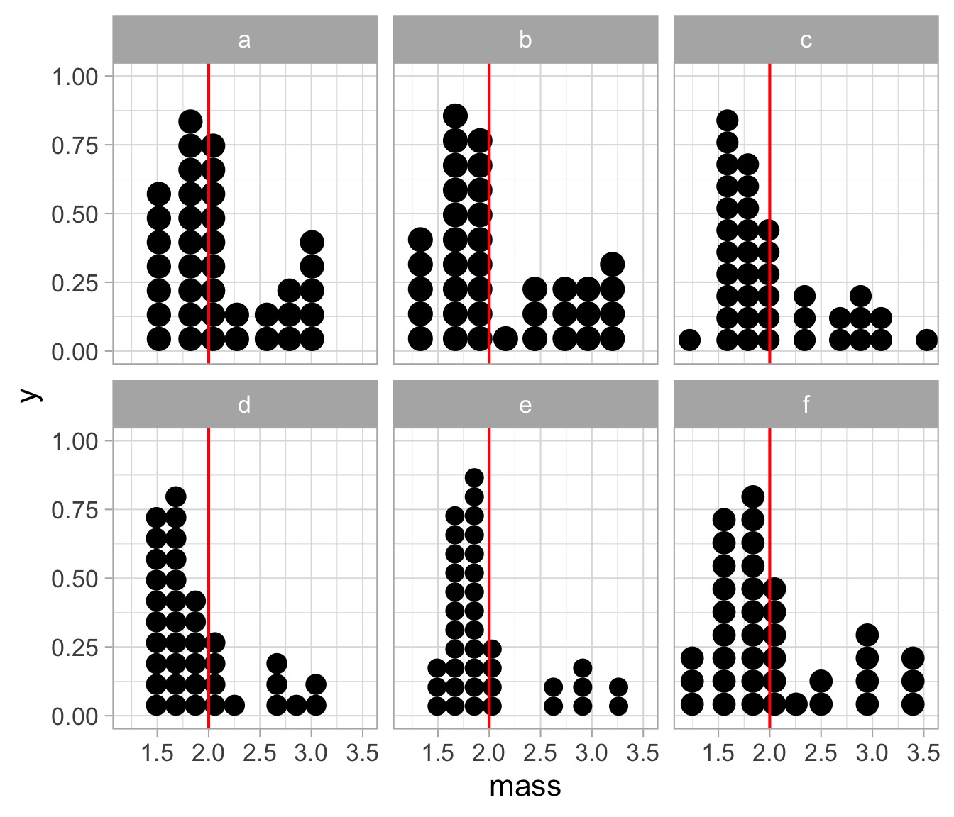
Visualizing Measures of Variability

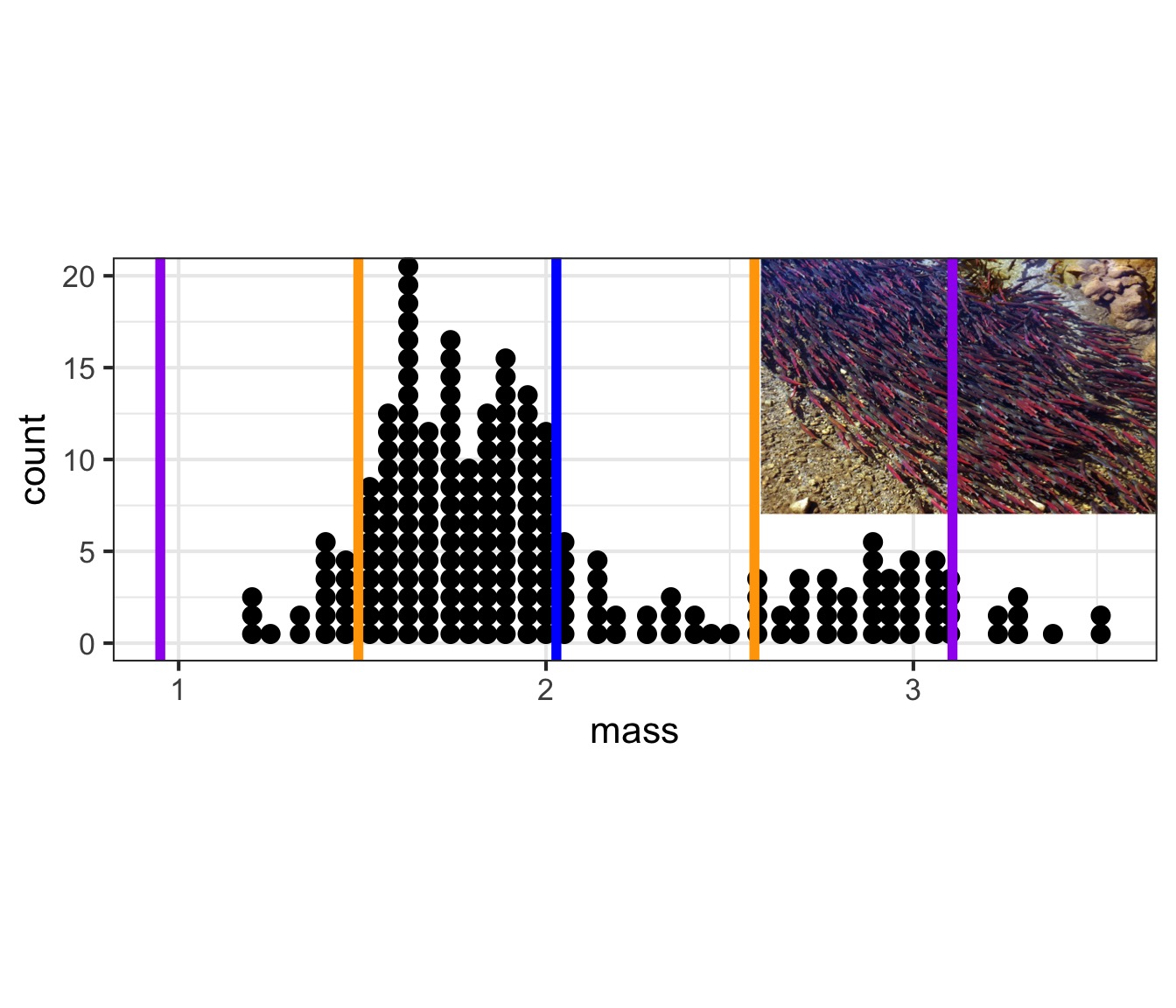
Variability: Quantiles/Percentiles and Quartiles

 [1] 1.56 1.61 1.76 2.16 2.69 2.88 2.91 2.98 3.06 3.09

    5%    10%    50%    90%    95% 
1.4270 1.5300 1.8550 2.9430 3.0865 

    0%    25%    50%    75%   100% 
1.1800 1.6400 1.8550 2.2675 3.5300 

Boxplots

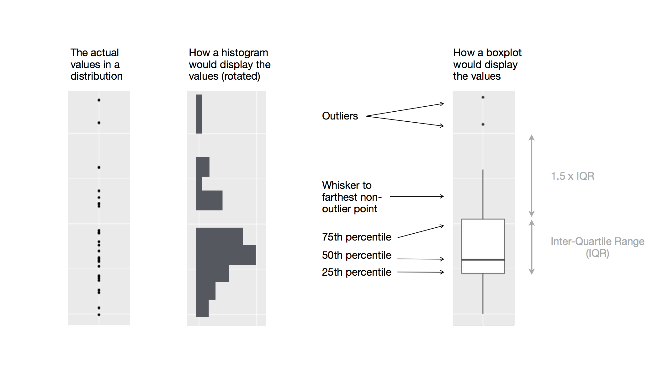
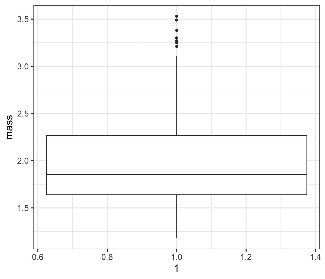
Boxplot of One Population

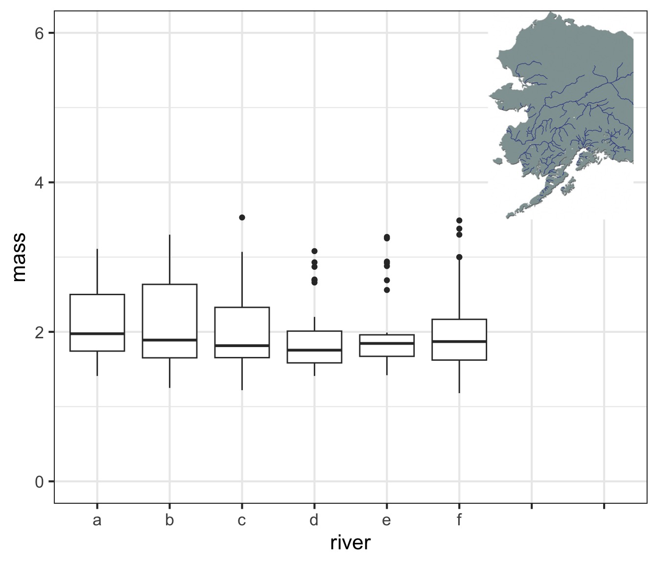
Boxplot of Many Populations

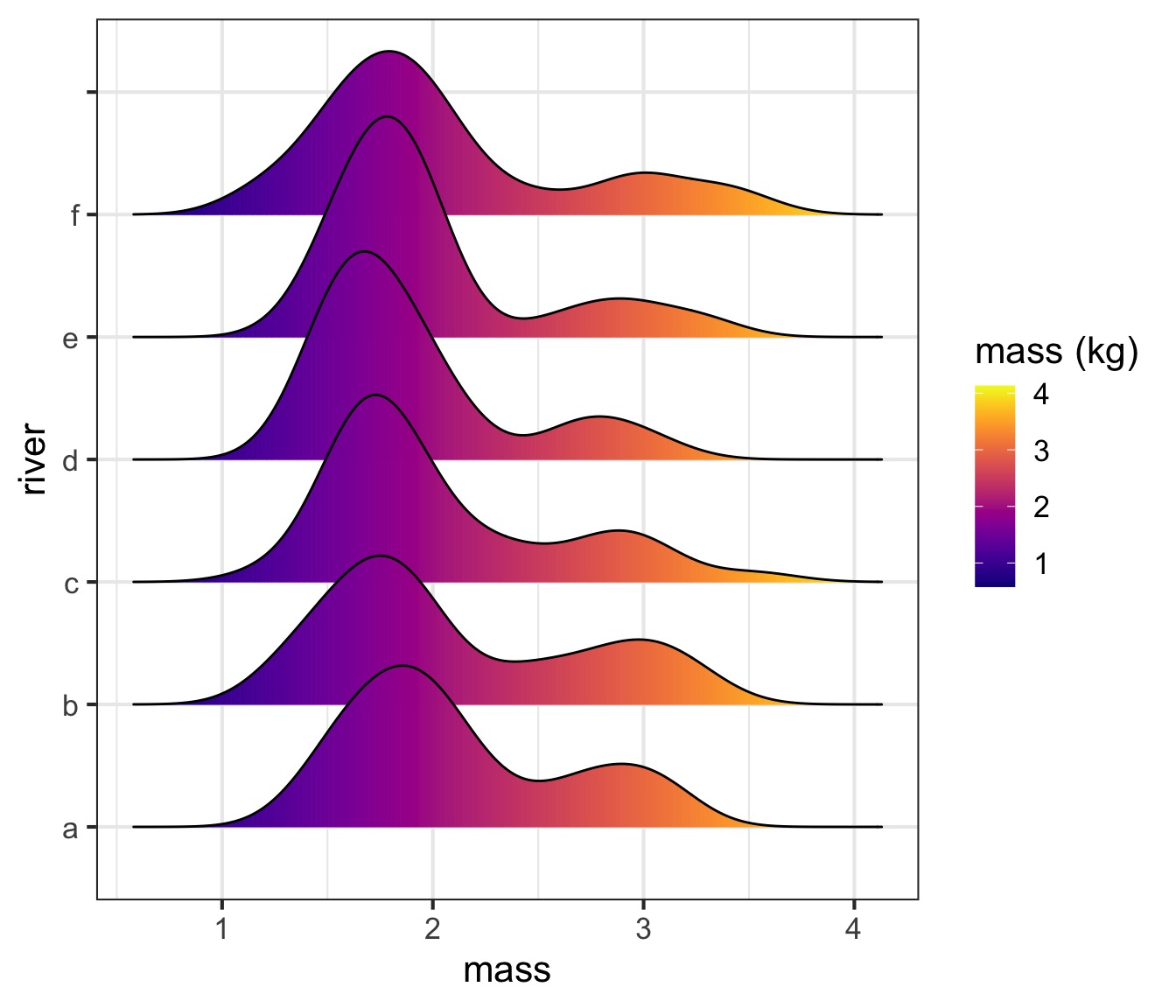
Meh, I still like ridgelines

Groups of Topics

1. Our Data

2. Cleaning and Filtering our Data

3. Summarizing counts functionally!

4. How do we summarize our data?

5. The split-apply-combine philosophy

Where are we going?

Split-Apply-Combine

• Filtering and working with one chunk of the data is not enough

• We often want to summarize information about many groups

Split-Apply-Combine

Two Questions

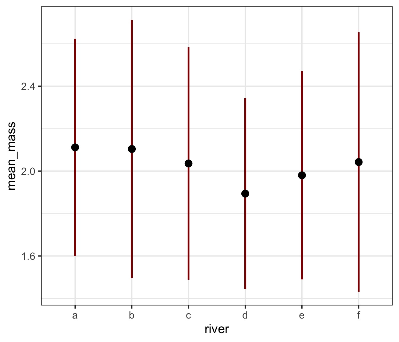
1. What is the mean and variation of salmon by river?

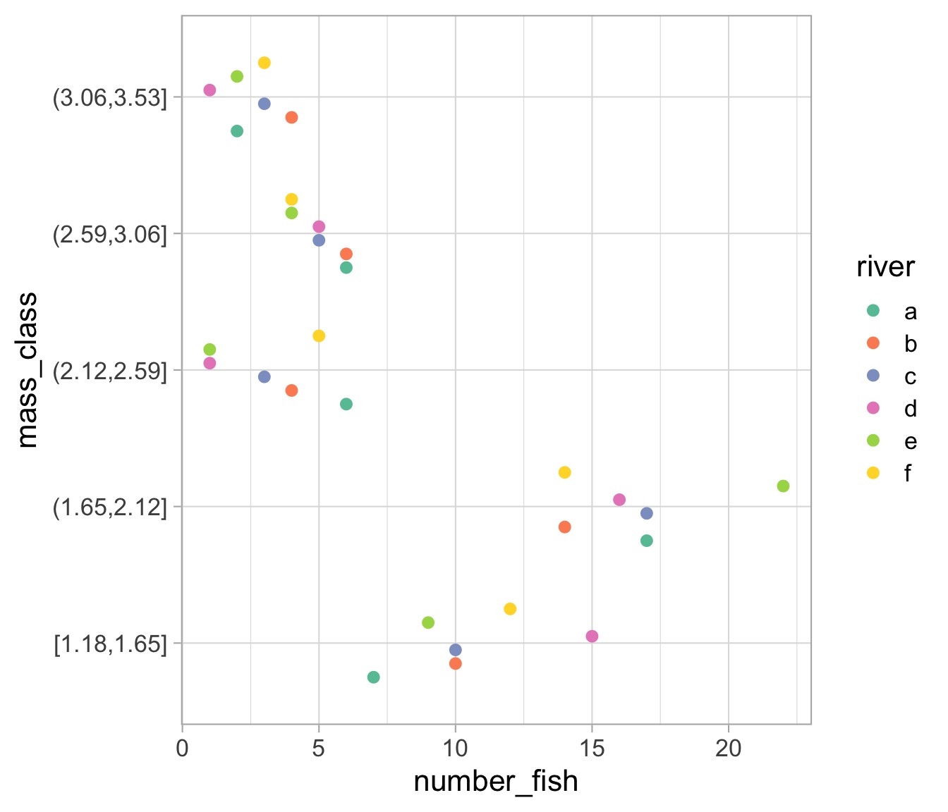
2. For each size class of salmon, how many are in each river?

What do we need to know to learn about rivers?

# make a data frame of summary info

  # start with data

  # group them (somehow?) by river

  # for each river, summarize the data to mean and sd

Start with the data

# make a data frame of summary info
salmon_rivers <- 
  
  # start with data
  salmon |>
  
  # group them (somehow?) by river

  # for each river, summarize the data to mean and sd

The group_by() function

# make a data frame of summary info
salmon_rivers <- 
  
  # start with data
  salmon |>
  
  # group them (somehow?) by river
  group_by(river)

  # for each river, summarize the data to mean and sd

Summarizing

# make a data frame of summary info
salmon_rivers <- 
  
  # start with data
  salmon |>
  
  # group them (somehow?) by river
  group_by(river) |>

  # for each river, summarize the data to mean and sd
  summarize(
    mean_mass = mean(mass),
    sd_mass = sd(mass)
  )

Show the result(yes, this could have been piped)

arrange(salmon_rivers, mean_mass)

# A tibble: 6 × 3
  river mean_mass sd_mass
  <chr>     <dbl>   <dbl>
1 d          1.89   0.450
2 e          1.98   0.491
3 c          2.04   0.548
4 f          2.04   0.612
5 b          2.10   0.608
6 a          2.11   0.511

Other way! Descending

arrange(salmon_rivers, desc(mean_mass))

# A tibble: 6 × 3
  river mean_mass sd_mass
  <chr>     <dbl>   <dbl>
1 a          2.11   0.511
2 b          2.10   0.608
3 f          2.04   0.612
4 c          2.04   0.548
5 e          1.98   0.491
6 d          1.89   0.450

What can we do with this?

What about mass class per river?

salmon_mass_count <- 
  
  # start with data
  salmon |>
  
  # make mass classes
  mutate(mass_class = cut_interval(mass, 5))

Mass Classes from cut_interval()

salmon_mass_count

# A tibble: 228 × 3
    mass river mass_class 
   <dbl> <chr> <fct>      
 1  3.09 a     (3.06,3.53]
 2  2.91 b     (2.59,3.06]
 3  3.06 c     (3.06,3.53]
 4  2.69 d     (2.59,3.06]
 5  2.88 e     (2.59,3.06]
 6  2.98 f     (2.59,3.06]
 7  1.61 a     [1.18,1.65]
 8  2.16 b     (2.12,2.59]
 9  1.56 c     [1.18,1.65]
10  1.76 d     (1.65,2.12]
# ℹ 218 more rows

OK, What next for count by class and river?

salmon_mass_count <- 
  
  # start with data
  salmon |>
  
  # make mass classes
  mutate(mass_class = cut_interval(mass, 5)) |>
  
  #.....

A Plan of Attack

salmon_mass_count <- 
  
  # start with data
  salmon |>
  
  # make mass classes
  mutate(mass_class = cut_interval(mass, 5)) |>
  
  # group by class and river
  
  # summarize with a count

Let’s do it with n()

salmon_mass_count <- 
  
  # start with data
  salmon |>
  
  # make mass classes
  mutate(mass_class = cut_interval(mass, 5)) |>
  
  # group by class and river
  group_by(mass_class, river) |>
  
  # summarize with a count
  summarize(number_fish = n())

Ungrouping to cleanup

salmon_mass_count <- 
  
  # start with data
  salmon |>
  
  # make mass classes
  mutate(mass_class = cut_interval(mass, 5)) |>
  
  # group by class and river
  group_by(mass_class, river) |>
  
  # summarize with a count
  summarize(number_fish = n()) |>
  
  ungroup()

Visualize our Result

A Solid Workflow!

If we have time - let’s see it live!

1. What are things you want to know about different rivers in the salmon data?

2. What are things you want to know about different size classes in the salmon data?